import logging

import matplotlib.pyplot as plt
import numpy as np
from jaxtyping import ArrayLike
from molmass import Formula
from scipy.constants import mega

from atmodeller import debug_logger
from atmodeller.classes import EquilibriumModel
from atmodeller.containers import (
    ChemicalSpecies,
    FixedFugacityConstraint,
    SpeciesNetwork,
    ThermodynamicState,
)
from atmodeller.interfaces import FugacityConstraintProtocol, ThermodynamicStateProtocol
from atmodeller.output import Output
from atmodeller.solubility import get_solubility_models

logger: logging.Logger = debug_logger()
logger.setLevel(logging.INFO)

Atmodeller initialized with double precision (float64)

Geological Outgassing

This notebook is available at notebooks/geological_outgassing.ipynb and is easiest to obtain by downloading the source code.

Atmodeller can perform “geological outgassing”, for example, as appears in Gaillard and Scaillet (2014). The model below reproduces the basic result of Gaillard and Scaillet (2014), Figure 3.

solubility_models = get_solubility_models()

# CO solubility neglected in Gaillard and Scaillet (low solubility in basaltic melt)
CO_g = ChemicalSpecies.create_gas("CO", solubility=solubility_models["CO_basalt_yoshioka19"])
O2_g = ChemicalSpecies.create_gas("O2")
CO2_g = ChemicalSpecies.create_gas("CO2", solubility=solubility_models["CO2_basalt_dixon95"])
H2_g = ChemicalSpecies.create_gas("H2", solubility=solubility_models["H2_basalt_hirschmann12"])
H2O_g = ChemicalSpecies.create_gas("H2O", solubility=solubility_models["H2O_basalt_mitchell17"])
# CH4 solubility neglected in Gaillard and Scaillet (low solubility in basaltic melt)
CH4_g = ChemicalSpecies.create_gas("CH4", solubility=solubility_models["CH4_basalt_ardia13"])
S2_g = ChemicalSpecies.create_gas("S2", solubility=solubility_models["S2_basalt_boulliung23"])
SO2_g = ChemicalSpecies.create_gas("SO2")
H2S_g = ChemicalSpecies.create_gas("H2S")
N2_g = ChemicalSpecies.create_gas("N2")

# Allow for graphite if stable, although the result demonstrates that graphite is not stable.
C_cr = ChemicalSpecies.create_condensed("C")

# Species lists for cases without nitrogen
species = SpeciesNetwork((CO_g, O2_g, CO2_g, H2_g, H2O_g, CH4_g, S2_g, SO2_g, H2S_g, C_cr))

model = EquilibriumModel(species)

[19:35:09 - atmodeller.classes             - INFO     ] - species_network = ('CO_g: IdealGas, _CO_basalt_yoshioka19', 'O2_g: IdealGas, NoSolubility', 'CO2_g: IdealGas, _CO2_basalt_dixon95', 'H2_g: IdealGas, SolubilityPowerLawLog10', 'H2O_g: IdealGas, SolubilityPowerLaw', 'CH4_g: IdealGas, _CH4_basalt_ardia13', 'S2_g: IdealGas, _S2_basalt_boulliung23', 'O2S_g: IdealGas, NoSolubility', 'H2S_g: IdealGas, NoSolubility', 'C_cd: CondensateActivity, NoSolubility')
[19:35:09 - atmodeller.classes             - INFO     ] - Thermodynamic data requires temperatures between 200 K and 6000 K
[19:35:09 - atmodeller.classes             - INFO     ] - reactions = {0: '1.0 CO2_g + 1.0 H2_g = 1.0 CO_g + 1.0 H2O_g',
 1: '2.0 CO_g + 2.0 H2_g = 1.0 CO2_g + 1.0 CH4_g',
 2: '2.0 CO2_g = 2.0 CO_g + 1.0 O2_g',
 3: '2.0 CO2_g + 0.5 S2_g = 2.0 CO_g + 1.0 O2S_g',
 4: '1.0 H2_g + 0.5 S2_g = 1.0 H2S_g',
 5: '2.0 CO_g = 1.0 CO2_g + 1.0 C_cd'}

Parameters from Gaillard and Scaillet (2014).

temperature_celsius = 1300
# Note that the Figure 3 inset box gives -1.4 but the caption gives -1.5
dlog10fO2_QFM = -1.5

temperature_K = temperature_celsius + 273.15

# The shift is quoted relative to FMQ, so use the online buffer calculator to convert to get the
# absolute FMQ in log10 units at 1300 C (https://fo2.rses.anu.edu.au/fo2app/)
# log10fO2 below is at temperature = 1302.04081632653 C at 1 bar
log10fO2 = -7.27787591128208

# Account for the shift to get the absolute fO2 in log10 units
log10fO2 += dlog10fO2_QFM

Take the nominal concentrations of C, H, and O from Gaillard and Scaillet (2014) and convert to masses.

# Initial volatile abundances (mole fraction) as estimated in undegassed Mid Ocean Ridge Basalts
CO2_initial = 600 / mega
H2O_initial = 1000 / mega
S_initial = 1000 / mega

# Approximate molar mass of basalt as pure SiO2, assuming some heavier and lighter components
# roughly cancel. A more accurate calculation could be performed if desired.
molar_mass_basalt = 60  # g/mol

# Mass fraction of volatiles per unit kg of basalt
C_mass = CO2_initial * Formula("C").mass / molar_mass_basalt
H_mass = H2O_initial * Formula("H2").mass / molar_mass_basalt
S_mass = S_initial * Formula("S").mass / molar_mass_basalt

logger.info("Mass of carbon = %0.5e", C_mass)
logger.info("Mass of hydrogen = %0.5e", H_mass)
logger.info("Mass of sulfur = %0.5e", S_mass)

[19:35:09 - atmodeller                     - INFO     ] - Mass of carbon = 1.20107e-04
[19:35:09 - atmodeller                     - INFO     ] - Mass of hydrogen = 3.35980e-05
[19:35:09 - atmodeller                     - INFO     ] - Mass of sulfur = 5.34413e-04

# Pressure range in bar, equivalent to Figure 3.
pressure_bar = np.logspace(-6, 3, num=100)
state: ThermodynamicStateProtocol = ThermodynamicState(temperature_K, pressure_bar)

# Impose the fO2 and volatile masses as constraints
fugacity_constraints: dict[str, FugacityConstraintProtocol] = {
    "O2_g": FixedFugacityConstraint(10**log10fO2)
}
mass_constraints: dict[str, ArrayLike] = {"C": C_mass, "H": H_mass, "S": S_mass}

model.solve(
    state=state,
    fugacity_constraints=fugacity_constraints,
    mass_constraints=mass_constraints,
    solver="basic",
)

output: Output = model.output
solution: dict[str, ArrayLike] = output.quick_look()

# Optionally, dump the data to Excel
# output.to_excel("gaillard")

[19:35:16 - atmodeller.classes             - INFO     ] - Solve (basic) complete: 100 (100.00%) successful model(s)
[19:35:16 - atmodeller.classes             - INFO     ] - Multistart summary: 100 (100.00%) models(s) required 1 attempt(s)
[19:35:17 - atmodeller.classes             - INFO     ] - Solver steps (max) = 94

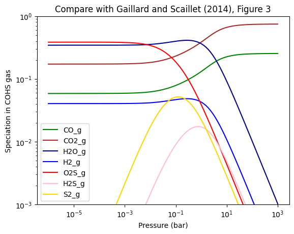
Plot the gas speciation to compare with Gaillard and Scaillet (2014), Figure 3.

# Get data as dataframes
data = output.to_dataframes()

# Plot total pressure on the x-axis
total_pressure = data["state"]["pressure"]

# Pick similar colours to Gaillard and Scaillet (2014) for easier visual comparison
colors = {
    "CO_g": "green",
    "CO2_g": "brown",
    "H2O_g": "darkblue",
    "H2_g": "blue",
    "O2S_g": "red",
    "H2S_g": "pink",
    "S2_g": "gold",
}

fig, ax = plt.subplots()

for species, color in colors.items():
    species_data = data[species]["volume_mixing_ratio"]
    ax.loglog(total_pressure, species_data, label=species, color=color)

ax.legend()
ax.set_title("Compare with Gaillard and Scaillet (2014), Figure 3")
ax.set_xlabel("Pressure (bar)")
ax.set_ylabel("Speciation in COHS gas")
ax.set_ylim(0.001, 1)

[19:35:19 - atmodeller.output_core         - INFO     ] - Computing to_dataframes output
[19:35:19 - atmodeller.output_core         - INFO     ] - Computing asdict output

(0.001, 1)